
Asana Data Revisited: Fall 2018 Semester In Review
I previously did a quick analysis of the data from Asana, the website I use to keep track of all my tasks.
Since it’s been about 6 months, I thought it would be interesting to take another look to see which trends remained and which changed.
import numpy as np
import pandas as pd
import matplotlib.pyplot as plt
import seaborn as sns
from plotly.offline import download_plotlyjs, init_notebook_mode, plot, iplot
import plotly.graph_objs as go
from plotly import tools
import cufflinks as cf
from wordcloud import WordCloud
import datetime
import collections
from lib import custom_utils

init_notebook_mode(connected=True)
cf.set_config_file(world_readable=True, offline=True)
[nltk_data] Downloading package stopwords to /home/sean/nltk_data...
[nltk_data]   Package stopwords is already up-to-date!
Notice I import a module called custom_utils. I recently started a project to keep track of my personal health and development and I found the need to reuse functions often. The file can be found here.
Data
Unlike last time, I’ll only be pulling the tasks related to school. Just before the start of last semester (Fall 2018), I created a new project using the Boards layout. This allows me to better organize my task by class.
First, let’s load that data.
f18_df = pd.read_csv('asana-umass-f18.csv', parse_dates=[1, 2, 3, 8, 9])
f18_df.head()
| Task ID | Created At | Completed At | Last Modified | Name | Column | Assignee | Assignee Email | Start Date | Due Date | Tags | Notes | Projects | Parent Task | |
|---|---|---|---|---|---|---|---|---|---|---|---|---|---|---|
| 0 | 949672124046393 | 2018-12-17 | 2018-12-19 | 2018-12-19 | training script to take only outputs for annot... | Research | NaN | NaN | NaT | NaT | NaN | NaN | UMass | NaN |
| 1 | 949607828976735 | 2018-12-17 | 2018-12-18 | 2018-12-18 | make generate preds output .npy file with pred... | Research | NaN | NaN | NaT | NaT | NaN | NaN | UMass | NaN |
| 2 | 949607828976733 | 2018-12-17 | 2018-12-18 | 2018-12-18 | option for generate preds script for not rotat... | Research | NaN | NaN | NaT | NaT | NaN | NaN | UMass | NaN |
| 3 | 949607828976731 | 2018-12-17 | 2018-12-18 | 2018-12-18 | make generate preds scripts output rboxes inst... | Research | NaN | NaN | NaT | NaT | NaN | NaN | UMass | NaN |
| 4 | 949607828976727 | 2018-12-17 | 2018-12-18 | 2018-12-18 | nms | Research | NaN | NaN | NaT | NaT | NaN | NaN | UMass | NaN |
Next, we can load the previous data to get some sweet comparison visualizations.
old_df = pd.read_csv('School.csv', parse_dates=[1, 2, 3, 7, 8])
old_df.tail()
| Task ID | Created At | Completed At | Last Modified | Name | Assignee | Assignee Email | Start Date | Due Date | Tags | Notes | Projects | Parent Task | |
|---|---|---|---|---|---|---|---|---|---|---|---|---|---|
| 804 | 351764138393835 | 2017-05-29 | 2017-05-30 | 2017-05-30 | brand new congress questions | NaN | NaN | NaT | NaT | NaN | NaN | School | NaN |
| 805 | 351764138393836 | 2017-05-29 | 2017-05-29 | 2017-05-29 | sign up for learnupon brand new congress | NaN | NaN | NaT | NaT | NaN | NaN | School | NaN |
| 806 | 351764138393838 | 2017-05-29 | 2017-06-28 | 2017-06-28 | create base for Hodler app | NaN | NaN | NaT | NaT | NaN | NaN | School | NaN |
| 807 | 351779687262554 | 2017-05-29 | 2017-06-28 | 2017-06-28 | battery life on lappy ubuntu | NaN | NaN | NaT | NaT | NaN | NaN | School | NaN |
| 808 | 356635261007682 | 2017-06-05 | 2017-06-28 | 2017-06-28 | bnc volunteer training | NaN | NaN | NaT | NaT | NaN | NaN | School | NaN |
all_df = pd.concat([old_df, f18_df], verify_integrity=True, ignore_index=True, sort=True)
all_df.head()
| Assignee | Assignee Email | Column | Completed At | Created At | Due Date | Last Modified | Name | Notes | Parent Task | Projects | Start Date | Tags | Task ID | |
|---|---|---|---|---|---|---|---|---|---|---|---|---|---|---|
| 0 | NaN | NaN | NaN | 2018-04-15 | 2018-04-15 | NaT | 2018-04-15 | More debt | NaN | NaN | School | NaT | NaN | 148623786710031 |
| 1 | NaN | NaN | NaN | 2018-04-07 | 2018-04-06 | NaT | 2018-04-07 | Send one line email to erik to add you to the ... | NaN | NaN | School | NaT | NaN | 148623786710030 |
| 2 | NaN | NaN | NaN | 2018-03-27 | 2018-03-27 | NaT | 2018-03-27 | withdraw from study abroad | NaN | NaN | School | NaT | NaN | 610060357624798 |
| 3 | NaN | NaN | NaN | 2018-03-26 | 2018-03-09 | NaT | 2018-03-26 | hold | NaN | NaN | School | NaT | NaN | 588106896688257 |
| 4 | NaN | NaN | NaN | 2018-02-23 | 2018-02-22 | 2018-02-23 | 2018-02-23 | find joydeep | NaN | NaN | School | NaT | NaN | 570162249229318 |
To help retain our sanity, let’s define colors for each semester.
all_color = 'rgba(219, 64, 82, 0.7)'
old_color = 'rgba(63, 81, 191, 1.0)'
f18_color = 'rgba(33, 150, 255, 1.0)'
Task Creation Day of Week Comparison
Let’s see if tasks where still created with the same daily frequencies. Since there are much more tasks in the old data, we can normalize the value counts for a fair comparison. For the sake of keeping the code clean and the x-axis in order, I decided keep the days of the week as numbers. For reference, 0 is Monday.
old_df['Created At DOW'] = old_df['Created At'].dt.dayofweek
f18_df['Created At DOW'] = f18_df['Created At'].dt.dayofweek
trace1 = go.Bar(
    x=old_df['Created At DOW'].value_counts(normalize=True).keys(),
    y=old_df['Created At DOW'].value_counts(normalize=True).values,
    name='Old Data',
    marker={
        'color': old_color
    }
)
trace2 = go.Bar(
    x=f18_df['Created At DOW'].value_counts(normalize=True).keys(),
    y=f18_df['Created At DOW'].value_counts(normalize=True).values,
    name='Fall 18',
    marker={
        'color': f18_color
    }
)

data = [trace1, trace2]
layout = go.Layout(
    barmode='group'
)

fig = go.Figure(data=data, layout=layout)
iplot(fig, filename='DOW Comparison')
This was quite a surprise. The days when I created tasks seems to have changed somewhat this semester.
Let’s check if the overall trend has remained the same.
all_df['Created At DOW'] = all_df['Created At'].dt.dayofweek

trace1 = go.Bar(
    x=all_df['Created At DOW'].value_counts(normalize=True).keys(),
    y=all_df['Created At DOW'].value_counts(normalize=True).values,
    name='All Data',
    marker={
        'color': all_color
    }
)

data = [trace1]
layout = go.Layout(
    barmode='group'
)

fig = go.Figure(data=data, layout=layout)
iplot(fig, filename='DOW Comparison')
There are definitely some small changes. Thursday caught up to Wednesday and Monday is catching up to Tuesday. However, the overall trend that I create the majority of my tasks at the beginning of the week remains strong.
Completion Time
Next, let’s look at the duration it took for me to complete each task. Because I used the parse_dates parameter when importing the CSVs, using the minus operator will return timedelta objects. Since Asana only provided dates without time, tasks with a duration of 0 days are ones that were created and completed on the same day.
Having already found outliers in the last analysis, let’s only consider only tasks that took less than 30 days to complete. Again, we normalize for a better comparison.
old_df['Duration'] = (old_df['Completed At'] - old_df['Created At'])
f18_df['Duration'] = (f18_df['Completed At'] - f18_df['Created At'])
trace1 = go.Bar(
    x=old_df[(old_df['Duration'].astype('timedelta64[D]') < 30)]['Duration'].value_counts(normalize=True).keys().days,
    y=old_df[(old_df['Duration'].astype('timedelta64[D]') < 30)]['Duration'].value_counts(normalize=True).values,
    name='Old Data',
    marker={
        'color': old_color
    }
)
trace2 = go.Bar(
    x=f18_df[(f18_df['Duration'].astype('timedelta64[D]') < 30)]['Duration'].value_counts(normalize=True).keys().days,
    y=f18_df[(f18_df['Duration'].astype('timedelta64[D]') < 30)]['Duration'].value_counts(normalize=True).values,
    name='Fall 18',
    marker={
        'color': f18_color
    }
)
data = [trace1, trace2]
layout = go.Layout(
    barmode='group'
)

fig = go.Figure(data=data, layout=layout)
iplot(fig, filename='grouped-bar')
Now this is interesting! For the most part, the time it takes me to complete tasks seems to have remained relatively the same. However, this semester it seems I create more tasks that take around a week to complete. In addition, I made less tasks that were completed on the same day.
Next, like last time, let’s see if we can figure out what type of tasks usually take longer to complete. I will once again use the fantastic word_cloud library by amueller.
# concatenate all name fields from tasks separated by duration of 3 days
old_less_text = ' '.join(list(old_df[old_df['Duration'].astype('timedelta64[D]') < 3]['Name'].dropna()))
old_grtr_text = ' '.join(list(old_df[old_df['Duration'].astype('timedelta64[D]') >= 3]['Name'].dropna()))

f18_less_text = ' '.join(list(f18_df[f18_df['Duration'].astype('timedelta64[D]') < 3]['Name'].dropna()))
f18_grtr_text = ' '.join(list(f18_df[f18_df['Duration'].astype('timedelta64[D]') >= 3]['Name'].dropna()))

# prep text
old_less_text = custom_utils.prep_text_for_wordcloud(old_less_text)
old_grtr_text = custom_utils.prep_text_for_wordcloud(old_grtr_text)

f18_less_text = custom_utils.prep_text_for_wordcloud(f18_less_text)
f18_grtr_text = custom_utils.prep_text_for_wordcloud(f18_grtr_text)

# get word frequencies
old_less_counts = dict(collections.Counter(old_less_text.split()))
old_grtr_counts = dict(collections.Counter(old_grtr_text.split()))

f18_less_counts = dict(collections.Counter(f18_less_text.split()))
f18_grtr_counts = dict(collections.Counter(f18_grtr_text.split()))

# create wordclouds
old_less_wordcloud = WordCloud(background_color="white", max_words=1000, margin=10,random_state=1).generate_from_frequencies(old_less_counts)
old_grtr_wordcloud = WordCloud(background_color="white", max_words=1000, margin=10,random_state=1).generate_from_frequencies(old_grtr_counts)

f18_less_wordcloud = WordCloud(background_color="white", max_words=1000, margin=10,random_state=1).generate_from_frequencies(f18_less_counts)
f18_grtr_wordcloud = WordCloud(background_color="white", max_words=1000, margin=10,random_state=1).generate_from_frequencies(f18_grtr_counts)

# display wordclouds using matplotlib
f, axes = plt.subplots(2, 2, sharex=True)
f.set_size_inches(18, 10)
axes[0, 0].imshow(old_less_wordcloud, interpolation="bilinear")
axes[0, 0].set_title('Old <3 days', fontsize=36)
axes[0, 0].axis("off")
axes[0, 1].imshow(old_grtr_wordcloud, interpolation="bilinear")
axes[0, 1].set_title('Old >=3 days', fontsize=36)
axes[0, 1].axis("off")

axes[1, 0].imshow(f18_less_wordcloud, interpolation="bilinear")
axes[1, 0].set_title('F18 <3 days', fontsize=36)
axes[1, 0].axis("off")
axes[1, 1].imshow(f18_grtr_wordcloud, interpolation="bilinear")
axes[1, 1].set_title('F18 >=3 days', fontsize=36)
axes[1, 1].axis("off")
(-0.5, 399.5, 199.5, -0.5)
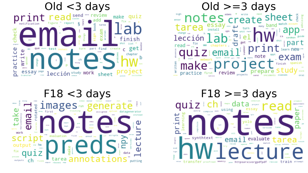
A few things changed this semester. The research project I was on during the semester was pretty demanding so a lot of those tasks show up like image, preds, or synthtext. Also, since none of my classes had projects this semester, that doesn’t show up.
However, some things remained the same. Homework usually takes more than 3 days and lecture notes are either done quickly or they get put off because other tasks are more important.
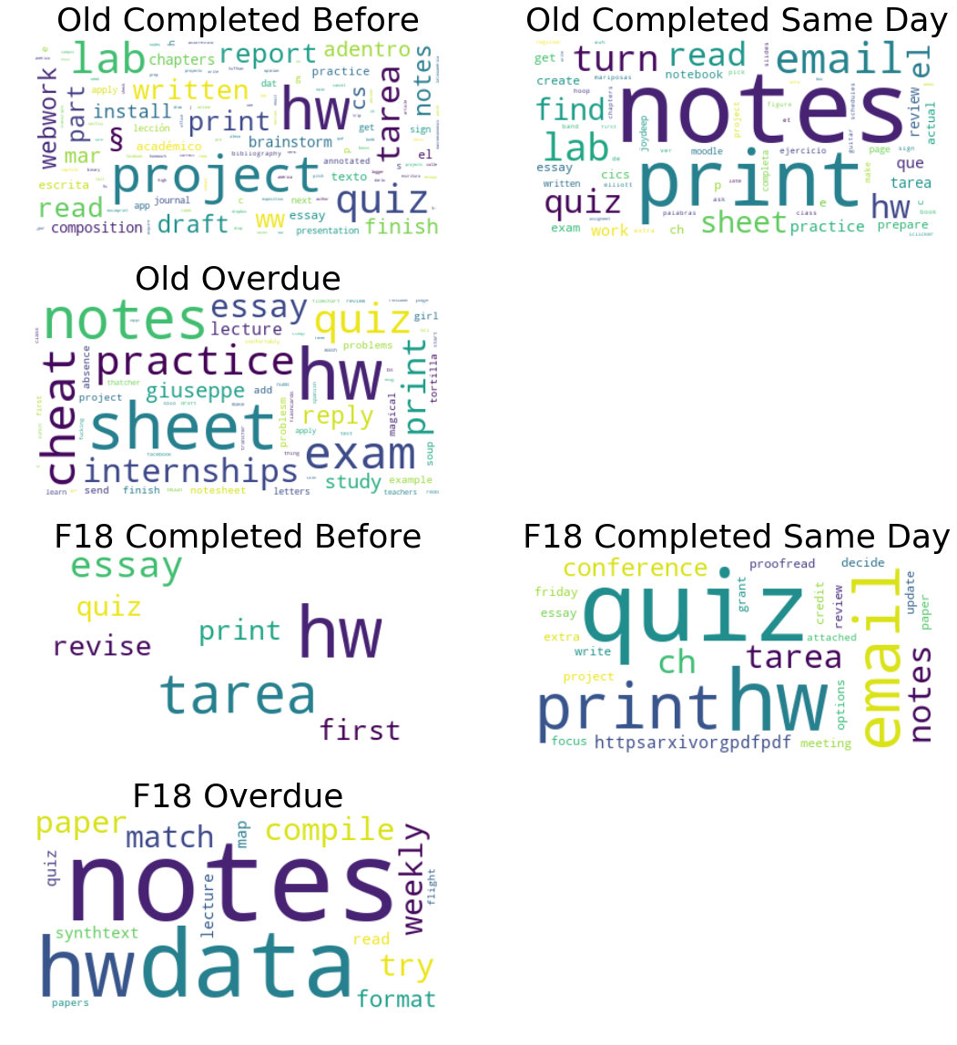
Overdue Tasks
Next, let’s take a look at overdue tasks.
old_df['Overdue'] = old_df['Completed At'] - old_df['Due Date']
f18_df['Overdue'] = f18_df['Completed At'] - f18_df['Due Date']
trace1 = go.Bar(
    x=old_df['Overdue'].value_counts(normalize=True).keys().days,
    y=old_df['Overdue'].value_counts(normalize=True).values,
    name='Old Data',
    marker={
        'color': old_color
    }
)
trace2 = go.Bar(
    x=f18_df['Overdue'].value_counts(normalize=True).keys().days,
    y=f18_df['Overdue'].value_counts(normalize=True).values,
    name='Fall 18',
    marker={
        'color': f18_color
    }
)
data = [trace1, trace2]
layout = go.Layout(
    barmode='group'
)

fig = go.Figure(data=data, layout=layout)
iplot(fig, filename='grouped-bar')
Seems like I did alright staying on top of things this semester.
Again, let’s use wordclouds to check out what might be causing me to miss due dates.
# concatenate all name fields from overdue tasks
old_before_text = ' '.join(list(old_df[old_df['Overdue'].astype('timedelta64[D]') < 0]['Name'].dropna()))
old_sameday_text = ' '.join(list(old_df[old_df['Overdue'].astype('timedelta64[D]') == 0]['Name'].dropna()))
old_overdue_text = ' '.join(list(old_df[old_df['Overdue'].astype('timedelta64[D]') > 0]['Name'].dropna()))

f18_before_text = ' '.join(list(f18_df[f18_df['Overdue'].astype('timedelta64[D]') < 0]['Name'].dropna()))
f18_sameday_text = ' '.join(list(f18_df[f18_df['Overdue'].astype('timedelta64[D]') == 0]['Name'].dropna()))
f18_overdue_text = ' '.join(list(f18_df[f18_df['Overdue'].astype('timedelta64[D]') > 0]['Name'].dropna()))

# prep text
old_before_text = custom_utils.prep_text_for_wordcloud(old_before_text)
old_sameday_text = custom_utils.prep_text_for_wordcloud(old_sameday_text)
old_overdue_text = custom_utils.prep_text_for_wordcloud(old_overdue_text)

f18_before_text = custom_utils.prep_text_for_wordcloud(f18_before_text)
f18_sameday_text = custom_utils.prep_text_for_wordcloud(f18_sameday_text)
f18_overdue_text = custom_utils.prep_text_for_wordcloud(f18_overdue_text)

# get word frequencies
old_before_counts = dict(collections.Counter(old_before_text.split()))
old_sameday_counts = dict(collections.Counter(old_sameday_text.split()))
old_overdue_counts = dict(collections.Counter(old_overdue_text.split()))

f18_before_counts = dict(collections.Counter(f18_before_text.split()))
f18_sameday_counts = dict(collections.Counter(f18_sameday_text.split()))
f18_overdue_counts = dict(collections.Counter(f18_overdue_text.split()))

# create wordclouds
old_before_wordcloud = WordCloud(background_color="white", max_words=1000, margin=10,random_state=1).generate_from_frequencies(old_before_counts)
old_sameday_wordcloud = WordCloud(background_color="white", max_words=1000, margin=10,random_state=1).generate_from_frequencies(old_sameday_counts)
old_overdue_wordcloud = WordCloud(background_color="white", max_words=1000, margin=10,random_state=1).generate_from_frequencies(old_overdue_counts)

f18_before_wordcloud = WordCloud(background_color="white", max_words=1000, margin=10,random_state=1).generate_from_frequencies(f18_before_counts)
f18_sameday_wordcloud = WordCloud(background_color="white", max_words=1000, margin=10,random_state=1).generate_from_frequencies(f18_sameday_counts)
f18_overdue_wordcloud = WordCloud(background_color="white", max_words=1000, margin=10,random_state=1).generate_from_frequencies(f18_overdue_counts)

# display wordclouds using matplotlib
f, axes = plt.subplots(4, 2, sharex=True)
f.set_size_inches(18, 20)
axes[0, 0].imshow(old_before_wordcloud, interpolation="bilinear")
axes[0, 0].set_title('Old Completed Before', fontsize=36)
axes[0, 0].axis("off")
axes[0, 1].imshow(old_sameday_wordcloud, interpolation="bilinear")
axes[0, 1].set_title('Old Completed Same Day', fontsize=36)
axes[0, 1].axis("off")
axes[1, 0].imshow(old_overdue_wordcloud, interpolation="bilinear")
axes[1, 0].set_title('Old Overdue', fontsize=36)
axes[1, 0].axis("off")
axes[1, 1].axis("off")

axes[2, 0].imshow(f18_before_wordcloud, interpolation="bilinear")
axes[2, 0].set_title('F18 Completed Before', fontsize=36)
axes[2, 0].axis("off")
axes[2, 1].imshow(f18_sameday_wordcloud, interpolation="bilinear")
axes[2, 1].set_title('F18 Completed Same Day', fontsize=36)
axes[2, 1].axis("off")
axes[3, 0].imshow(f18_overdue_wordcloud, interpolation="bilinear")
axes[3, 0].set_title('F18 Overdue', fontsize=36)
axes[3, 0].axis("off")
axes[3, 1].axis("off")
(-0.5, 399.5, 0.0, 1.0)
Busiest Class this Semester
Since I began to track the class for each task, we can check out which class was my busiest this semester.
# https://community.plot.ly/t/setting-up-pie-charts-subplots-with-an-appropriate-size-and-spacing/5066
domain1={'x': [0, 1], 'y': [0, 1]}#cell (1,1)

fig = {
  "data": [
    {
      "values": f18_df['Column'].value_counts().values,
      "labels": f18_df['Column'].value_counts().keys(),
      'domain': domain1,
      "name": "Fall 18",
      "hoverinfo":"label+percent+name",
      "hole": .4,
      "type": "pie"
    }],
  "layout": {
        "annotations": [
            {
                "font": {
                    "size": 15
                },
                "showarrow": False,
                "text": "Fall 2018",
                "x": 0.5,
                "y": 0.5
            }
        ]
    }
}

iplot(fig, filename='donut')
Due Date Frequency this Semester
We can also see when my tasks were due.
trace1 = go.Bar(
    x=f18_df['Due Date'].dropna().value_counts().keys(),
    y=f18_df['Due Date'].dropna().value_counts().values,
    name='Fall 18',
    marker={
        'color': f18_color
    }
)

data = [trace1]
iplot(data, filename='due date freq')
Conclusion
Hopefully this post show the motivation and potential benefit of revisiting a previous analysis in an attempt to find any significant changes. In the context of personal development, doing so can help you track your progress and achieve your goals. I still definitely need to put more effort into taking notes on time!