
Quick Exploration of Asana Data
If you have never heard of it, Asana is a pretty neat tool for keeping track of your personal tasks or managing the Agile workflow of a team. Here’s what their landing pages says:
Asana is the easiest way for teams to track their work—and get results.
Since I’ve been using it for about three years now, I would say that statement is pretty accurate. Recently, it dawned on me the amount of potential insights data from Asana could provide about my productivity. Sure enough, there is an “Export to CSV” but in the actions menu (click the down arrow next to the project name in the center of the screen) for every project!
Let’s see what lies in my (un)productivity data…
import numpy as np
import pandas as pd
import matplotlib.pyplot as plt
import seaborn as sns
from plotly.offline import download_plotlyjs, init_notebook_mode, plot, iplot
import plotly.graph_objs as go
from plotly import tools
import cufflinks as cf
from wordcloud import WordCloud
import nltk
import re
import string

nltk.download('stopwords')
cachedStopWords = nltk.corpus.stopwords.words("english")
punct = set(string.punctuation)

init_notebook_mode(connected=True)
cf.set_config_file(world_readable=True, offline=True)
[nltk_data] Downloading package stopwords to /home/sean/nltk_data...
[nltk_data]   Package stopwords is already up-to-date!
For my own sanity, I split my tasks into two projects: School for school related tasks and, Tasks for everything else. My Personal Tasks is the default personal tasks project and is what I used before I created the Tasks project.
Let’s import the CSVs and concatenate them. I use the verify_integrity to make sure there aren’t any duplicates from shifting tasks between projects.
df1 = pd.read_csv('School.csv', parse_dates=[1, 2, 3, 7, 8])
df2 = pd.read_csv('Tasks.csv', parse_dates=[1, 2, 3, 7, 8])
df3 = pd.read_csv('My_Personal_Tasks.csv', parse_dates=[1, 2, 3, 7, 8])
frames = [df1, df2, df3]
df = pd.concat(frames, verify_integrity=True, ignore_index=True)
df.head()
| Task ID | Created At | Completed At | Last Modified | Name | Assignee | Assignee Email | Start Date | Due Date | Tags | Notes | Projects | Parent Task | |
|---|---|---|---|---|---|---|---|---|---|---|---|---|---|
| 0 | 148623786710031 | 2018-04-15 | 2018-04-15 | 2018-04-15 | More debt | NaN | NaN | NaT | NaT | NaN | NaN | School | NaN |
| 1 | 148623786710030 | 2018-04-06 | 2018-04-07 | 2018-04-07 | Send one line email to erik to add you to the ... | NaN | NaN | NaT | NaT | NaN | NaN | School | NaN |
| 2 | 610060357624798 | 2018-03-27 | 2018-03-27 | 2018-03-27 | withdraw from study abroad | NaN | NaN | NaT | NaT | NaN | NaN | School | NaN |
| 3 | 588106896688257 | 2018-03-09 | 2018-03-26 | 2018-03-26 | hold | NaN | NaN | NaT | NaT | NaN | NaN | School | NaN |
| 4 | 570162249229318 | 2018-02-22 | 2018-02-23 | 2018-02-23 | find joydeep | NaN | NaN | NaT | 2018-02-23 | NaN | NaN | School | NaN |
df['Projects'].value_counts(dropna=False)
School          766
Tasks           321
NaN             160
Hampstead WX     17
Name: Projects, dtype: int64
I found interesting that the My Personal Tasks pulled in some tasks from an archived project called Hampstead WX. That project was a site I created a while ago.
Here I plot a histogram of the day of the week the tasks were created on.
dayOfWeek={0:'Mon', 1:'Tue', 2:'Wed', 3:'Thu', 4:'Fri', 5:'Sat', 6:'Sun'}
df['Created At DOW'] = df['Created At'].dt.dayofweek.map(dayOfWeek)
x = []
y = []
for key, day in dayOfWeek.items():
    x.append(day)
    y.append(df['Created At DOW'].value_counts()[day])
bar_tracer = [go.Bar(x=x, y=y)]
iplot(bar_tracer)
I can’t say I didn’t expect these results. The bulk of my tasks are created at the start of the week and they slowly fade off until Saturday.
Next, let’s look at the duration it took for me to complete each task. Because I used the parse_dates parameter when importing the CSVs, using the minus operator will return timedelta objects. Since Asana only provided dates without time, tasks with a duration of 0 days are ones that were created and completed on the same day.
df['Duration'] = (df['Completed At'] - df['Created At'])
x = df['Duration'].value_counts().keys().days
y = list(df['Duration'].value_counts().values)
bar_tracer = [go.Bar(x=x, y=y)]
iplot(bar_tracer)
Wow! Seems like we have some outliers. Let’s see what some of them are.
df[df['Duration'].astype('timedelta64[D]') > 75]
| Task ID | Created At | Completed At | Last Modified | Name | Assignee | Assignee Email | Start Date | Due Date | Tags | Notes | Projects | Parent Task | Created At DOW | Duration | |
|---|---|---|---|---|---|---|---|---|---|---|---|---|---|---|---|
| 151 | 425397822367084 | 2017-09-08 | 2017-12-19 | 2017-12-19 | Comp Sci 220 | NaN | NaN | NaT | NaT | NaN | NaN | School | NaN | Fri | 102 days |
| 166 | 425397822367086 | 2017-09-08 | 2017-12-21 | 2017-12-21 | Comp Sci 240 | NaN | NaN | NaT | NaT | NaN | NaN | School | NaN | Fri | 104 days |
| 184 | 425397822367087 | 2017-09-08 | 2017-12-19 | 2017-12-19 | Physics 151 | NaN | NaN | NaT | NaT | NaN | NaN | School | NaN | Fri | 102 days |
| 296 | 425397822367083 | 2017-09-08 | 2017-12-19 | 2017-12-19 | Stats 515 | NaN | NaN | NaT | NaT | NaN | NaN | School | NaN | Fri | 102 days |
| 344 | 177397329054805 | 2016-09-06 | 2017-07-26 | 2017-07-26 | Misc: | NaN | NaN | NaT | NaT | NaN | NaN | School | NaN | Tue | 323 days |
| 362 | 148623786709961 | 2017-01-26 | 2017-07-24 | 2017-07-24 | al dimeola - egyptian danza LISTEN AND LEARN | NaN | NaN | NaT | NaT | NaN | NaN | School | NaN | Thu | 179 days |
| 419 | 200785803637408 | 2016-10-23 | 2017-07-26 | 2017-07-26 | watch shit | NaN | NaN | NaT | NaT | NaN | howls moving castle\nnausicaa\nyeh jawaani hai... | School | NaN | Sun | 276 days |
| 512 | 177397329054770 | 2016-09-06 | 2017-05-18 | 2017-05-18 | NaN | NaN | NaN | NaT | NaT | NaN | NaN | School | NaN | Tue | 254 days |
| 540 | 177397329054778 | 2016-09-06 | 2017-05-18 | 2017-05-18 | NaN | NaN | NaN | NaT | NaT | NaN | NaN | School | NaN | Tue | 254 days |
| 638 | 177397329054780 | 2016-09-06 | 2017-05-18 | 2017-05-18 | NaN | NaN | NaN | NaT | NaT | NaN | NaN | School | NaN | Tue | 254 days |
| 668 | 179665031917793 | 2016-09-12 | 2017-05-18 | 2017-05-18 | NaN | NaN | NaN | NaT | NaT | NaN | NaN | School | NaN | Mon | 248 days |
| 692 | 177397329054776 | 2016-09-06 | 2017-05-18 | 2017-05-18 | NaN | NaN | NaN | NaT | NaT | NaN | NaN | School | NaN | Tue | 254 days |
| 724 | 207879281133328 | 2016-11-06 | 2017-02-15 | 2017-02-15 | figure out piano chords from HATE verses | NaN | NaN | NaT | NaT | NaN | NaN | School | NaN | Sun | 101 days |
| 733 | 201648184747252 | 2016-10-24 | 2017-01-23 | 2017-01-23 | transcribe good voice recordings | NaN | NaN | NaT | NaT | NaN | NaN | School | NaN | Mon | 91 days |
| 734 | 201648184747254 | 2016-10-24 | 2017-02-15 | 2017-02-15 | transcribe dank part from Skin Deep | NaN | NaN | NaT | NaT | NaN | NaN | School | NaN | Mon | 114 days |
| 1058 | 432400137331715 | 2017-09-18 | 2017-12-07 | 2017-12-07 | hit up Ben for the db seeds | NaN | NaN | NaT | NaT | NaN | NaN | Tasks | NaN | Mon | 80 days |
| 1238 | 95110234477969 | 2016-02-27 | 2016-07-05 | 2016-07-05 | Switch to google charts | Sean Kelley | seangtkelley@gmail.com | NaT | NaT | NaN | NaN | Hampstead WX | NaN | Sat | 129 days |
From what I can tell, about half of these are not actually tasks but rather sections. Asana interestingly still allows you to mark a section as complete which is why my sections for classes like Comp Sci 220 and Stats 515 show up.
The others are a mixed bag. A lot are music projects I was working that obviously took a while. Another task was a global task I had with a running list of all the movies I need to watch.
Let’s go deeper into the histogram. Here, I split the bars by their respective project and only look at the tasks that took less than 30 days to complete.
trace1 = go.Bar(
    x=df[(df['Duration'].astype('timedelta64[D]') < 30) & (df['Projects'] == 'School')]['Duration'].value_counts().keys().days,
    y=df[(df['Duration'].astype('timedelta64[D]') < 30) & (df['Projects'] == 'School')]['Duration'].value_counts().values,
    name='School'
)
trace2 = go.Bar(
    x=df[(df['Duration'].astype('timedelta64[D]') < 30) & (df['Projects'] == 'Tasks')]['Duration'].value_counts().keys().days,
    y=df[(df['Duration'].astype('timedelta64[D]') < 30) & (df['Projects'] == 'Tasks')]['Duration'].value_counts().values,
    name='Tasks'
)
data = [trace1, trace2]
layout = go.Layout(
    barmode='group'
)

fig = go.Figure(data=data, layout=layout)
iplot(fig, filename='grouped-bar')
It seems between both projects, the distribution of the tasks is very similar. Most tasks are completed within the two weeks after creation. This result definitely highlights the intended purpose of Asana (or at least how I use it). Personally, any deadline that is more than a month away I usually put in Google Calendar, rather than create a task in Asana.
Next, let’s see if we can figure out what type of tasks usually take longer to complete. I will once again use the fantastic word_cloud library by amueller.
# concatenate all name fields from tasks separated by duration of 3 days
less_text = ' '.join(list(df[df['Duration'].astype('timedelta64[D]') < 3]['Name'].dropna()))
grtr_text = ' '.join(list(df[df['Duration'].astype('timedelta64[D]') >= 3]['Name'].dropna()))

# remove any punctuation
less_text = ''.join(ch for ch in less_text if ch not in punct)
grtr_text = ''.join(ch for ch in grtr_text if ch not in punct)

# remove stopwords
less_text = ' '.join([word for word in less_text.split() if word not in cachedStopWords])
grtr_text = ' '.join([word for word in grtr_text.split() if word not in cachedStopWords])

# create wordclouds
less_wordcloud = WordCloud(background_color="white", max_words=1000, margin=10,random_state=1).generate(less_text)
grtr_wordcloud = WordCloud(background_color="white", max_words=1000, margin=10,random_state=1).generate(grtr_text)

# display wordclouds using matplotlib
f, (ax1, ax2) = plt.subplots(1, 2, sharex=True)
f.set_size_inches(18, 5)
ax1.imshow(less_wordcloud, interpolation="bilinear")
ax1.set_title('<3 days', fontsize=36)
ax1.axis("off")
ax2.imshow(grtr_wordcloud, interpolation="bilinear")
ax2.set_title('>=3 days', fontsize=36)
ax2.axis("off")
(-0.5, 399.5, 199.5, -0.5)
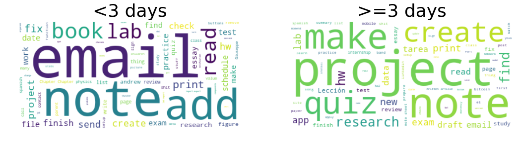
This is by far my favorite visualization. Right away we can see the difference between long and short term tasks.
Some of the top words for the less than three days category are email, note, add, read, and print. Each of these tasks are relatively simple and usually require at most a few actions.
Some of the top words for the greater than or equal to three days category are project, quiz, note, create, make, and research. In contrast, each one of these tasks evidently require more effort and take a lot longer.
It’s interesting that note was a top word in both wordclouds. I can only assume that notes are not high priority for me so they are equally likely to be done immediately or postponed.
Next, let’s take a look at overdue tasks. I haven’t started putting due dates on tasks until recently so there isn’t as much good data but we’ll work with what we’ve got.
Like the Duration field, I again use the timedelta functionality for the datetime objects. In this case, positive deltas will represent tasks completed after the due date and negative deltas tasks completed before the due date.
df['Overdue'] = df['Completed At'] - df['Due Date']
trace1 = go.Bar(
    x=df[(df['Projects'] == 'School')]['Overdue'].value_counts().keys().days,
    y=df[(df['Projects'] == 'School')]['Overdue'].value_counts().values,
    name='School'
)
trace2 = go.Bar(
    x=df[(df['Projects'] == 'Tasks')]['Overdue'].value_counts().keys().days,
    y=df[(df['Projects'] == 'Tasks')]['Overdue'].value_counts().values,
    name='Tasks'
)
data = [trace1, trace2]
layout = go.Layout(
    barmode='group'
)

fig = go.Figure(data=data, layout=layout)
iplot(fig, filename='grouped-bar')
I was happy to see that for the most part, I complete tasks before their set due dates.
Let’s do a similar wordcloud analysis of the overdue tasks to see what might be causing the delay in completion. Here, I’m going to split the tasks into three sections: completed more than one day before due date, completed on same day as due date, and completed after due date.
# concatenate all name fields from overdue tasks
before_text = ' '.join(list(df[df['Overdue'].astype('timedelta64[D]') < 0]['Name'].dropna()))
sameday_text = ' '.join(list(df[df['Overdue'].astype('timedelta64[D]') == 0]['Name'].dropna()))
overdue_text = ' '.join(list(df[df['Overdue'].astype('timedelta64[D]') > 0]['Name'].dropna()))

# remove any punctuation
before_text = ''.join(ch for ch in before_text if ch not in punct)
sameday_text = ''.join(ch for ch in sameday_text if ch not in punct)
overdue_text = ''.join(ch for ch in overdue_text if ch not in punct)

# remove stopwords
before_text = ' '.join([word for word in before_text.split() if word not in cachedStopWords])
sameday_text = ' '.join([word for word in sameday_text.split() if word not in cachedStopWords])
overdue_text = ' '.join([word for word in overdue_text.split() if word not in cachedStopWords])

# create wordclouds
before_wordcloud = WordCloud(background_color="white", max_words=1000, margin=10,random_state=1).generate(before_text)
sameday_wordcloud = WordCloud(background_color="white", max_words=1000, margin=10,random_state=1).generate(sameday_text)
overdue_wordcloud = WordCloud(background_color="white", max_words=1000, margin=10,random_state=1).generate(overdue_text)

# display wordclouds using matplotlib
f, ((ax1, ax2), (ax3, ax4)) = plt.subplots(2, 2, sharex=True)
f.set_size_inches(18, 10)
ax1.imshow(before_wordcloud, interpolation="bilinear")
ax1.set_title('Completed Before', fontsize=36)
ax1.axis("off")
ax2.imshow(sameday_wordcloud, interpolation="bilinear")
ax2.set_title('Completed Same Day', fontsize=36)
ax2.axis("off")
ax3.imshow(overdue_wordcloud, interpolation="bilinear")
ax3.set_title('Overdue', fontsize=36)
ax3.axis("off")
ax4.axis("off")
(-0.5, 399.5, 0.0, 1.0)
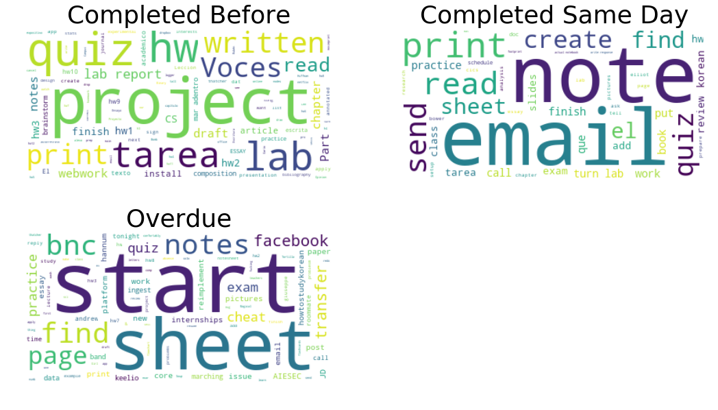
As expected, we some similar words to those in the Duration analysis but there are also some new ones.
In the completed before wordcloud, the words tarea and Voces come up which are actually Spanish for homework and Voices respectively. I study Spanish at University and for some reason, I always write tarea instead of homework just for homework in my Spanish classes. And Voces was the name of a latin american poetry textbook we had one semester in which we often had reading assignments.
Probably the most revealing worldcloud is the overdue one. It’s clear that I have a problem with starting tasks.
Conclusion
Hopefully this post shows just a glimpse of the insights you can gleen from diving into your own metadata. Many productivity applications have options for downloading your data in bulk and I would implore you to give it a shot. Perhaps you can use your discoveries to improve your work habits to become or lifestyle!