Extended Autoregressive Rollout of Prithvi-WxC AI Weather Model

Introduction to Artificial Intelligence Weather Prediction (AIWP) Models

Artificial Intelligence Weather Prediction (AIWP) models are starting to represent a new paradigm in weather forecasting. Without going into the details, rather than relying on traditional physics-based numerical simulations, these models are entirely data-driven, requiring vast datasets to learn how to forecast the weather.

For example, GraphCast from Google DeepMind was trained on ERA5 from ECMWF and Prithvi WxC from NASA and IBM was trained on MERRA-2 from NASA.

These reanalysis datasets are created by using data assimilation techniques, combining forecast ensembles and observations, to create reconstructions of atmospheric variables. In essence, these reanalyses represent our best understanding of state of the atmosphere at given times.

Data Biases

This data-intensive approach will inevitably be vulnerable to biases which exist in the datasets. For example, initial research has shown that if historical tropical cyclones are removed from the dataset, AIWPs will no longer be able to properly predict any cyclone events.

In this blog post, I’ll detail my basic experimental setup to investigate the hypothesis that these models have learned a tendency to warm over time in accordance with how climate change is reflected in the reanalysis training datasets.

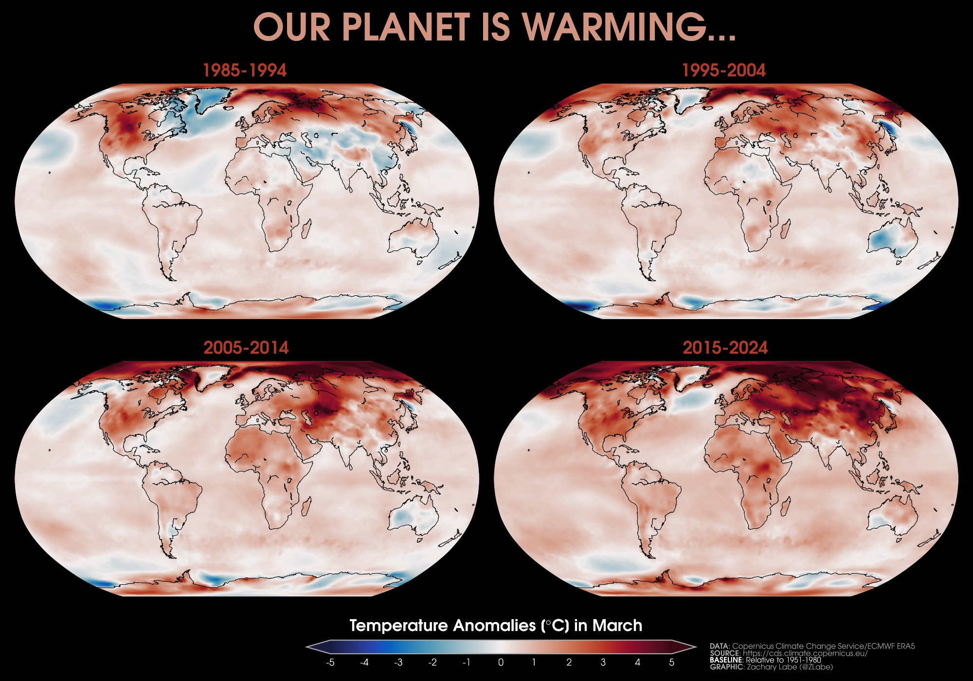Depiction of warming temperatures in ERA5 dataset by Zack Labe

Prithvi-WxC

NASA and IBM teamed up to create Prithvi-WxC, a foundational model designed not just for weather but for broader Earth system predictions. It can be fine-tuned for various downstream applications including weather forecasting, downscaling, and gravity wave parameterization.

A huge benefit is that the model code is available on GitHub and the weights are openly available on Hugging Face, making it more accessible for researchers and developers. This openness makes it quite easy for anyone to play with the model and contrasts with other state-of-the-art models that are locked behind institutional barriers.

What Happens to Predictions Past Normal Forecast Domain?

The Prithvi-WxC repository includes an example notebook for using a version of Prithvi-WxC fine-tuned for autoregressive rollout. Autoregressive rollout in this context means the sucessesive use of model output to generate further output. This could be considered somewhat analygus to weather forecasting where, starting from an initial state of the atmosphere, the model first predicts the state 6 hours in the future. Then, it uses that 6 hour prediction to advance another 6 hours, producing a 12 hour preduction, etc.

Prithvi-WxC, like many models in this domain of weather forecasting, is optimized for short-term forecasts or even nowcasts, typically not much longer than a 48-hour window. But what if we extend this autoregressive rollout further, beyond what it was trained for? Since the model is trained on data with a rising temperature trend, does it project that same trend forward?

If so, it would be a good indication that these data-driven models cannot be directly used for long-term climate modeling using simple autoregressive techniques.

Experimental Setup

Starting from the example notebook as a base, I made some modifications to allow for extended autoregression. I won’t go into the nitty-gritty details, but here is a summary:

Autoregression is controlled by the input_time and lead_time variables, where input_time is the initial state fed to the model and lead_time is the target time to forecast. Both are measured in hours, input_time is negative, and lead_time must be a positive multiple of input_time. By default, the example notebook forecasts 12 hours into the future with a 6 hour timestep: input_time = -6 and lead_time = 12.

The Merra2RolloutDataset dataloader then uses the input_time and lead_time with an additional parameter time_range to obtain surface, vertical, and climatology data which is used to enhance rollout performance. time_range is expected to be a tuple with the beginning and ending timestamps which correspond with the input_time and lead_time.

From the notebook:

When performing auto-regressive rollout, the intermediate steps require the static data at those times and—if using residual=climate—the intermediate climatology. We provide a dataloader that extends the MERRA2 loader of the core model, adding in these additional terms. Further, it return target data for the intermediate steps if those are required for loss terms.

and

The PrithviWxC model was trained to calculate the output by producing a perturbation to the climatology at the target time. This mode of operation is set via the residual=climate option. This was chosen as climatology is typically a strong prior for long-range prediction. When using the residual=climate option, we have to provide the dataloader with the path of the climatology data.

Since only data for 2020 is available in the Hugging Face repository for Prithvi-WxC and we want to push the rollout past data observed by the model, we will have to get creative.

In my most successful experiment, I used the following configuration to initialize the dataloader:

time_range = ("2020-01-01T00:00:00", "2021-01-01T00:00:00")
input_time = -24*30
lead_time = abs(input_time)*11

from PrithviWxC.dataloaders.merra2_rollout import Merra2RolloutDataset

dataset = Merra2RolloutDataset(
    time_range=time_range,
    lead_time=lead_time,
    input_time=input_time,
    data_path_surface=surf_dir,
    data_path_vertical=vert_dir,
    climatology_path_surface=surf_clim_dir,
    climatology_path_vertical=vert_clim_dir,
    surface_vars=surface_vars,
    static_surface_vars=static_surface_vars,
    vertical_vars=vertical_vars,
    levels=levels,
    positional_encoding=positional_encoding,
)
assert len(dataset) > 0, "There doesn't seem to be any valid data."

This will gather the relevant data for the beginning of each month throughout 2020 to correspond with one month autoregressive steps. Thus, dataset.nsteps is 11 corresponding with lead_time. However, in the autoregressive loop, I introduce a separate variable nsteps_extended to be the actual amount of autoregressive steps we want to advance into the future.

In my code below, in choose to attempt to go 10 years with nsteps_extended = (24*365*10)//abs(input_time). Then, I add a modulo (%) operator on lines that require nsteps e.g. batch["climate"] = batch["climates"][:, step % nsteps]. Since I’m trying to push past the available data, this modulo will essentially allow the autoregressive loop to wrap around once the data runs out. So in the case above, with nsteps equivalent to 1 year and nsteps_extended equivalent to 10 years, predictions past 2020 will continue to use the 2020 initialization data.

This is obviously not ideal, but it is a result of how the model is designed to be rolled out, at least from my understanding and the examples available. I would argue that climatology data does not change on short time scales, so using one year’s climatology should be relatively consistent across multiple years. But I will concede it is a flaw in this experiment.

Finally, I saved model outputs as checkpoints Google Drive which allowed me to continue rollout from where it left off when Colab kicks me off the runtime for inactivity.

Here is the autoregressive loop code which is modified from rollout.py:

nsteps_extended = (24*365*10)//abs(input_time) # ten years
nsteps = dataset.nsteps

steps_per_checkpoint = 1

import time

# main autoregression loop
rng_state_1 = torch.get_rng_state()

with torch.no_grad():
    model.eval()

    # attempt to load last checkpoint
    checkpoints = [f.name for f in checkpoint_path.iterdir() if f.is_file()]
    print(f"Checkpoints: {checkpoints}")
    if len(checkpoints) > 0:
      get_chkpt_num = lambda x: int(x.split(".")[0].split("_")[-1])
      checkpoints = sorted(checkpoints, key=get_chkpt_num)
      last_checkpoint = checkpoints[-1]
      print(f"Loading checkpoint: {last_checkpoint}")

      batch["x"] = torch.load(checkpoint_path / last_checkpoint).to(device)
      xlast = batch["x"][:, -1] # `out` from the previous run concated on line below
      start_step = get_chkpt_num(last_checkpoint)+1
    else:
      print("No checkpoints found, starting from scratch")
      xlast = batch["x"][:, 1]
      start_step = 0

    batch["lead_time"] = batch["lead_time"][..., 0]

    # Save the masking ratio to be restored later
    mask_ratio_tmp = model.mask_ratio_inputs

    for step in range(start_step, nsteps_extended):
        print(f"Starting step {step}/{nsteps_extended}...")

        # start time
        t0 = time.time()

        # After first step, turn off masking
        if step > 0:
            model.mask_ratio_inputs = 0.0

        # modulo step based on nsteps to cyclically take from
        # available data. normally for loop above would exit
        # at nsteps, but since we're pushing it, we need to
        # wrap around
        batch["static"] = batch["statics"][:, step % nsteps]
        batch["climate"] = batch["climates"][:, step % nsteps]
        batch["y"] = batch["ys"][:, step % nsteps]

        out = model(batch)

        batch["x"] = torch.cat((xlast[:, None], out[:, None]), dim=1)
        xlast = out

        # save checkpoint
        print(f"{step}/{nsteps_extended}")
        if step % steps_per_checkpoint == 0:
          print(f"Saving checkpoint {step}...")
          torch.save(batch["x"], checkpoint_path / f'step_{step}.pt')

        # end time
        t1 = time.time()
        print(f"Step {step} took {t1-t0} seconds")

    # Restore the masking ratio
    model.mask_ratio_inputs = mask_ratio_tmp

The table below shows a brief comparison of how inference time increases dramatically with longer timesteps.

Results

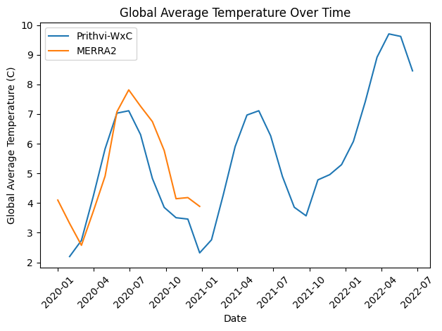Results of extended autoregressive rollout from Jan 2020 to July 2022

Above is a plot comparing the predicted global average temperature from the extended rollout to the MERRA2 ground truth. Unfortunately, I was only able to obtain the MERRA2 data for 2020 as it was easily available in the Hugging Face repository for Prithvi-WxC as mentioned above.

The model seems to do quite well for 2020, although the second half of the year is where skill begins to drop off. Prithvi-WxC underestimates the temperature by a considerable margin. This may not be unexpected as some AIWP models have shown a cold bias.

There does seem to be a small warming trend, however, there is not nearly enough data here to making any concrete statements. This trend could simply be natural variation or a model anomaly.

Next Steps and Future Improvements

Finish Plot with MERRA2 Data for Entire Domain

The analysis would be much improved if the plot included MERRA2 data to compare to Prithvi-WxC output up to July 2022. This would be a relatively easy step in code terms, but could be very costly in the time and disk space to download the MERRA2 NetCDF4 files.

Finish Extended Rollout to 10 Years

I tried a few times to continue rollout from the last checkpoint produced from the run which produced the plot above, but Google Collab would simply not advance. I’m not sure what the exact issue was, but it would have been ideal to go the full 10 years to properly identify a trend.

Determine the Fastest and Most Reliable Timestep for Extended Rollout

As shown in the inference time comparison table, larger timesteps take much more time to inference. By testing a range of values on just a few rollout steps, estimated time to complete the full rollout could be calculated and compared to find the optimal value for quickest rollout.

Experiment with Better Experimental Design

This experiment was more of a personal interest of mine rather than hard science. I’d love to design a more robust experiment that more directly isolates the climate signal in long-term predictions made by AIWP models.

Conclusion

Data-driven, ML approaches have truly sparked a revolution in the fields of meteorology and climatology. Foundational models like Prithvi-WxC are just example and hopefully through this blog post I’ve shown how easy it is for anyone to experiment with them. Was I able to show that global warming was inadvertently learned during training? Not quite, but this line of inquiry regarding implicit data biases should remain prescient with data-hungry approaches like modern deep learning.

Currently, ML is also providing fresh approaches for disciplines across the domain including data assimilation, subgrid parameterization, downscaling, and bias correction. Scientists should retain a healthy level of skepticism and aspire to rigorously test new methods, especially before they are operationalized. We must also be conscious of the emissions released from training and using these models. However, these models should not be ignored as the potential for transformative application is substantial.

Appendix

Results Code

1. Parallelize calculation of global average temperature from saved model checkpoints

import concurrent.futures
import torch
from tqdm import tqdm

def process_checkpoint(index, checkpoint_file):
    checkpoint = torch.load(checkpoint_file)
    global_avg_temp = checkpoint[:, -1, 12].mean().item()
    return index, global_avg_temp

checkpoint_files = list(checkpoint_path.glob("*.pt"))
global_avg_temps = [None] * len(checkpoint_files)

with concurrent.futures.ThreadPoolExecutor() as executor:
    futures = [executor.submit(process_checkpoint, i, checkpoint_file) for i, checkpoint_file in enumerate(checkpoint_files)]
    for future in tqdm(concurrent.futures.as_completed(futures), total=len(futures)):
        index, global_avg_temp = future.result()
        global_avg_temps[index] = global_avg_temp

2. Assemble dataframe of corresponding timestamps

import pandas as pd

start_datetime = datetime.strptime(time_range[0], "%Y-%m-%dT%H:%M:%S") + timedelta(hours=abs(input_time))
timestamps = [start_datetime]
current_datetime = start_datetime
for i in range(len(global_avg_temps)-1):
  current_datetime += timedelta(hours=abs(input_time) * steps_per_checkpoint)
  timestamps.append(current_datetime)

df = pd.DataFrame({'timestamp': timestamps, 'global_avg_temp': global_avg_temps})
df['timestamp'] = pd.to_datetime(df['timestamp'])
df['global_avg_temp'] = df['global_avg_temp'] - 273.15

3. Get available MERRA-2 reanalysis temps for comparison

import os
from glob import glob

import xarray as xr

merra2_sfc_files = glob(os.path.join(os.path.abspath(surf_dir), "*_sfc_*.nc"))

merra2_dates = []
merra2_global_means = []
for filepath in merra2_sfc_files:
  try:
    # get the date of the file from the filename
    date_str = filepath.split("/")[-1].split(".")[0].split("_")[-1]
    merra2_dates.append(datetime.strptime(date_str, "%Y%m%d"))

    ds = xr.open_dataset(filepath)

    # query the dataset for the T2M variable
    merra2_global_means.append(ds.T2M.mean() - 273.15)

    ds.close() # Important to close the dataset
  except Exception as e:
    print(f"Error loading {filepath}: {e}")
merra2_df = pd.DataFrame({'timestamp': merra2_dates, 'merra2_global_means': merra2_global_means})

4. Plot results

import matplotlib.pyplot as plt

plt.plot(df.timestamp, df.global_avg_temp, label="Prithvi-WxC")
plt.plot(merra2_df.timestamp, merra2_df.merra2_global_means, label="MERRA2")
plt.legend()
plt.xlabel("Date")
plt.ylabel("Global Average Temperature (C)")
plt.title("Global Average Temperature Over Time")
plt.xticks(rotation=45)
plt.tight_layout()
plt.show()